

Biological Evolution and Information Acquisition
A few weeks ago we looked at a simulation of technological evolution by economist Brian Arthur, in which he was able to start with simple building blocks (such as a NAND gate) and evolve surprisingly complex circuits (such as a 12-way AND gate or a 4-bit adder) by randomly combining increasingly useful existing components. We analyzed this as a way of simplifying a search problem: by using existing, working components as modules that can be combined, a few at a time, into more complex modules, and then combining those into even more complex modules, many unpromising and time-consuming branches of the search tree are screened off, and the simulation can find useful technologies amidst an enormous branching set of possibilities.
Real human technology is, of course, not generated by randomly combining components together and seeing if they do anything useful; the randomness in these simulations is just a way to see how easy or hard it is to create new technologies under different conditions. But biological technology — the huge panoply of lifeforms that exist on earth, from microscopic single-celled organisms to whales the size of a 737 — is also generated by randomness. Evolution builds biological technology bit by bit by harvesting the fruits of genetic variation, often caused by random mutation, preferentially selecting the most fit organisms to propagate their genes into the future. Over billions of years, this process can generate astoundingly complex biological systems.
What’s interesting is that biological evolution uses a very similar trick to Arthur’s circuit simulation. By leveraging modularity at the genetic level, populations of organisms can increase the rate that useful genetic variants spread through the population, effectively increasing their rate of information acquisition. Sexual reproduction, along with other ways of sharing genetic material like horizontal gene transfer, is essentially a mechanism for doing this. We can show this with some simple simulations.
Evolution and reproductive strategies
The simplest way for an organism to reproduce is asexual reproduction, where a parent produces a child that’s a genetic copy of itself. Simple single-celled organisms, for instance, reproduce by cellular fission, dividing into two or more “children” that each have the same genes as the original parent.
But children won’t necessarily be identical copies of their parents. Due to genetic mutation, some genes might get randomly altered during the fission process, producing children with slightly different genes. In some cases, these mutations might be useful, giving additional functionality such as antibiotic resistance and thus better odds of surviving and reproducing. Because of their contribution to the organism’s fitness, over time the useful mutations will become more and more common in the population.
We can demonstrate this with a simple simulation. In our simulation, we start with a population of 100 creatures, each of which has a genome of 200 individual genes. A gene can either be a 1 (the “good” version of the gene) or a 0 (the “bad” version of the gene). The initial population is random, with each creature having roughly a 50-50 mix of good and bad genes. Each iteration of the simulation, each creature produces two children. A child copies the genes of its parent, but due to mutation each gene has a 0.2% chance of being flipped, going from a 1 to a 0 or vice versa. The 100 most fit children (where fitness is just the sum of each gene value, since 1 is the “good” version of the gene in our simplified model) are selected to continue the next generation, and the cycle repeats. This is a simplification compared to how evolution actually functions — for one, it treats genes as contributing to fitness independently, ignoring the fact that the fitness value of one gene often depend on other genes — but it’s enough to show some of the dynamics at work.
When we run this simulation, the proportion of “good” genes in the population steadily rises over time as more-fit offspring outcompete less-fit offspring. Depending on the mutation rate, the population may eventually reach maximum possible fitness of 200, or plateau at some level below it.
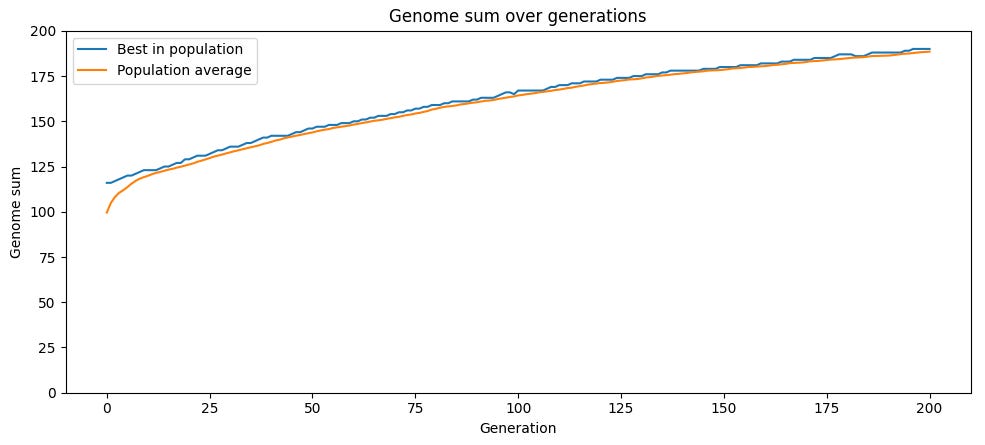
The problem with this strategy — producing children that are noisy copies of a single parent, and relying purely on random mutation as a source of genetic variation — is that once you’re at above-average fitness, mutations are likely to be bad on average. If a genome has more 1s than 0s, a random change will be more likely to change a 1 to a 0 than a 0 to a 1. Thus for parents of above-average fitness, their children will on average have lower fitness.
Because mutation is random, there will nonetheless be variation, and some children will end up with higher fitness than their parents. And because selection eliminates the least fit each iteration, the pool of selected children will have higher average fitness than their parents, allowing average fitness to increase over time. But mutation reducing average fitness drags down this process.
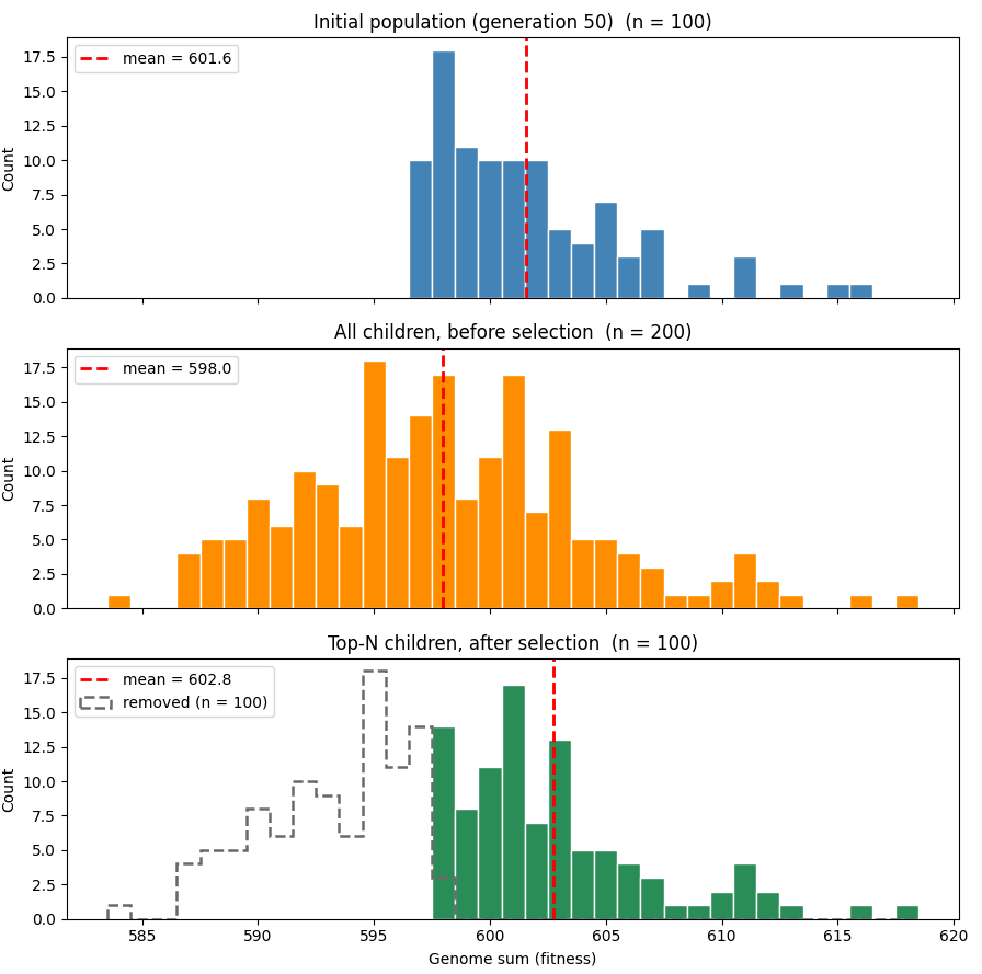
You can see this in the graph below, which shows a simulation with slightly different parameters (a genome length of 1000 and a mutation rate of 2%) to more easily see the trends. The top graph shows the distribution of population fitness at generation 50, and the second graph shows the distribution of the population’s children prior to selection. You can see that, thanks to mutation, average fitness has dropped, though due to randomness some proportion of the children have lucked into getting higher fitness. The last graph shows the children after the top half of the distribution has been selected. Average fitness rises, and is now above the initial population, though just barely.
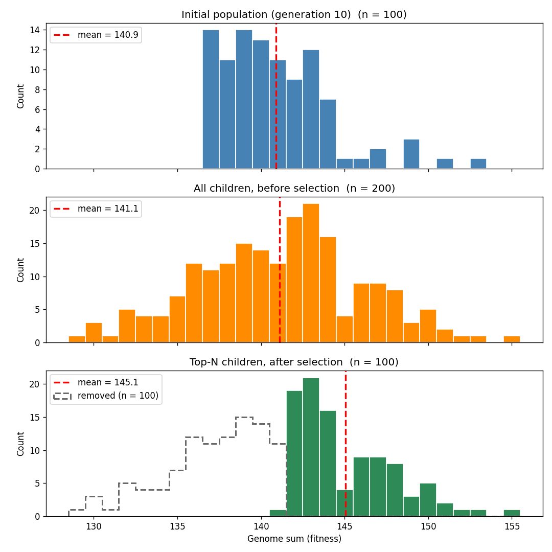
Now let’s look at a simulation of a different reproductive strategy: sexual reproduction, where children get their genes from two parents rather than just one. In this simulation, we still have a population of 100 creatures with genomes of 200 genes, each of which can either be a 0 or a 1. But now children have two parents, and in each iteration members of the population are paired up randomly and each pair produces four children. Children get their genes from both parents with each gene having a 50% chance of coming from a particular parent. The top 100 most fit children are then selected for the next generation, and the iteration continues. In this simulation, there is no mutation, so genetic variation entirely comes from reshuffling the genes of the parents.
Like the previous simulation, the population gradually reaches maximum fitness. But sexual reproduction gets there much faster. With asexual reproduction, after 200 generations the population was around an average fitness of 187. With sexual reproduction, the population average reached the fitness maximum of 200 in just 33 generations.
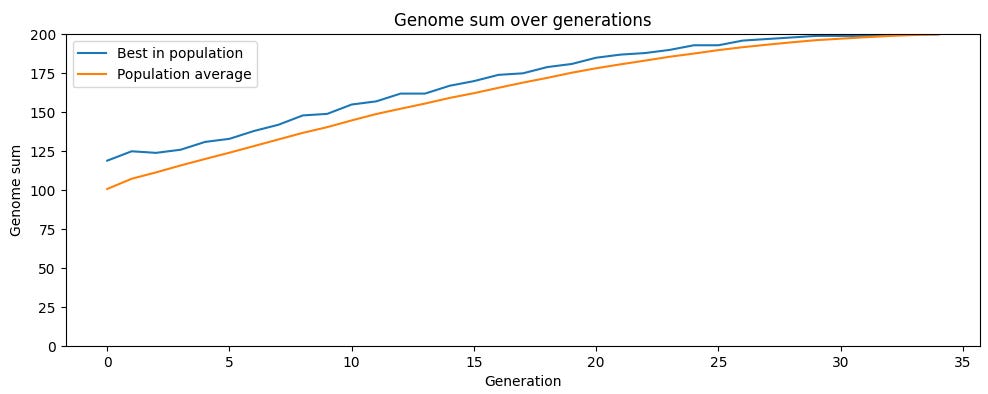
The key is that sexual reproduction introduces genetic variation without reducing average fitness. Since children are a random combination of their parents’ genes, on average they’ll have the same fitness as their parents (with some randomly having higher fitness, and others randomly having lower fitness). When the most-fit children are selected for the next generation, this is taking the top half of a distribution with a much higher average than the distribution of children in the asexual simulation. Average fitness thus rises much faster.
If you work out the math (or, as I did, simply read the math that someone else worked out), in an asexual population the rate of fitness increase is 1/(8*f), where f is the differential normalized fitness. (The normalized fitness of a population is the average fraction of good genes in that population; so a population where, on average, a member has 150 good genes in a genome of 200 would have a normalized fitness of 0.75. Differential normalized fitness is the normalized fitness of the population minus 0.5, the normalized fitness of a randomly generated population.) Early on, fitness of a population can increase quickly, but the rate soon drops below an increase of 1 unit of fitness per generation (one gene flipped from a 0 to a 1 on average). As a population gets closer to maximum possible fitness, the rate of fitness increase approaches 0.25 (flipping one gene, on average, from a 0 to a 1 every four generations).
With sexual reproduction, on the other hand, the rate of fitness increase turns out to be much higher: it’s proportional to the square root of the length of the genome.
The informational power of genetic recombination
One way to think about why sexual reproduction is so powerful is to look at lineages of descent. Say that one of the members of our asexually reproducing population stumbles across a new, useful mutation. Because genes are passed from one parent to one child, the only way this gene can spread throughout the population (in the absence of some other member of the population also stumbling across it) is if the children of whoever has it outcompete the children of everyone else. In this scenario, the population eventually ends up consisting entirely of descendants of one particular member of the population — as a necessary condition of this spread, every other genetic lineage (along with whatever useful mutations they might have stumbled across) gets wiped out.
We can see this in our simulation results. The chart below assigns each member of the initial population, and their children, a unique color. The simulation starts out with 100 different colors (one for each member of the population), but this quickly gets winnowed down to a much smaller number. After a few generations, the population is one uniform color, all descendents of one particular member of the initial population. (This chart is from one particular simulation run, but repeated runs will show the same behavior.)
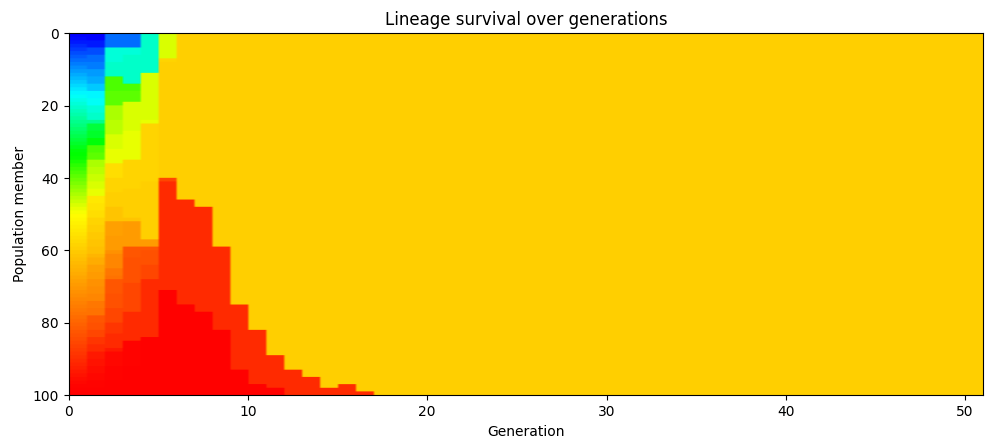
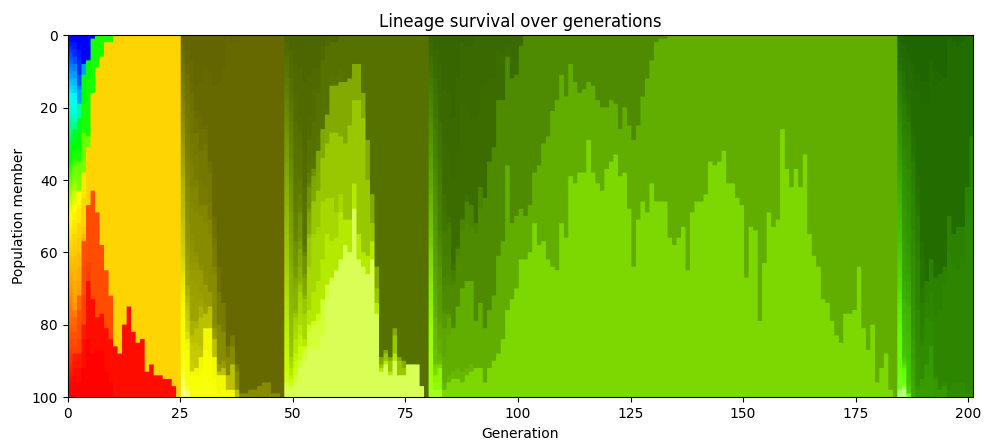
If we redo the color coding whenever the population reaches the point where everyone is descended from a single ancestor, we see that this happens repeatedly. In the chart below, the population at generation 48 are all descendants of one particular member of the population who lived in generation 25. At generation 80, they’re all descendants of one particular member alive from generation 48.
In evolutionary biology, this phenomenon is known as “clonal interference”: if two different beneficial mutations arise in different members of the population of the same generation they can’t be shared and so they end up competing against each other, and one beneficial mutation ultimately gets wiped out.
With a sexually reproducing population, on the other hand, useful mutations can be shared much more easily. In an asexual population, a member has one parent, one grandparent, one great-grandparent, and so on. But in a sexual population, a member has two parents, four grandparents, eight great-grandparents, etc. Beneficial variation from earlier generations can spread much more easily.
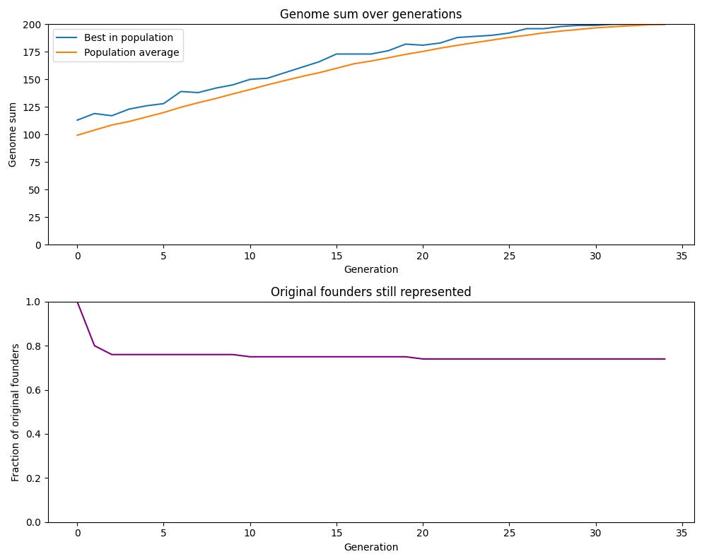
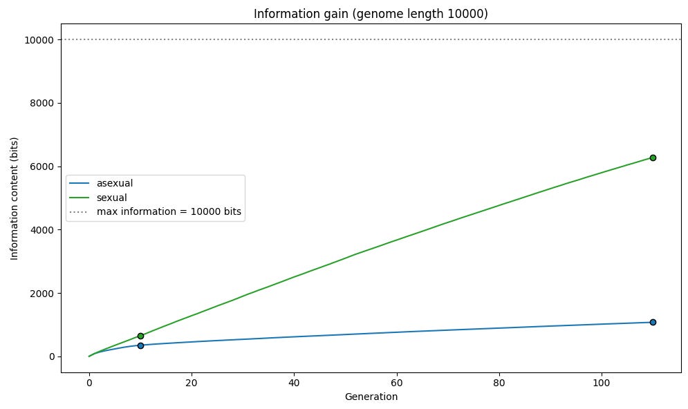
We can see this in the graph below, which shows the proportion of genes of the original members of a sexually reproducing population represented in the gene pool at any given time. We can see that the proportion stays very high: genes from almost 75% of the original population are found in the population after 34 generations. In the asexual population, this was 1% (and would be even lower in larger populations, since it’s just 1/total starting population).
We previously noted that Brian Arthur’s circuit simulation took advantage of modularity, finding useful subcomponents, locking in their designs, and then using those to build more complex technologies. Once the simulation finds a 3-way AND gate, it can use that to make a 4-way AND gate, which it can use to make a 5-way AND gate. We likewise noted that if you’re trying to build an 8-bit adder by randomly combining NAND gates together, it’s vastly easier if you can add one NAND gate at a time and verify you’re correct than if you have to guess all 68 gates at once.
You can think of this like someone solving a combination lock. A lock with a five-digit combination, with 100 possible values for each digit, has 100^5 = 10 billion possible combinations. Trying combinations one by one would take forever.
Technological modularity is like being a skilled lockpick that can check whether each individual digit attempted on a combination is correct (maybe by listening carefully you can hear a telltale “click” when the dial is in the right spot). Now instead of searching over 10 billion possible combinations, you’re doing five searches over 100 possible values each, or 500 possibilities total. The space of possible options that must be considered is vastly reduced.
Sexual reproduction is, as I understand it, doing something similar: by letting genes from two parents be combined to form children, it effectively lets the fitness of each gene be tested independently, turning the search from something like “find the best 200-gene genome” to something closer to 200 parallel “find the best gene at this location” searches. In our combination lock analogy, the modular circuit simulation is sort of like turning the dial until you hear a “click,” which indicates that the given number is correct. Sexual reproduction is more like trying a bunch of different random combinations, getting back a score for “how close this combination is to being solved,” and using that to infer which “dials” are correct. The search space is correspondingly greatly narrowed, and the search proceeds much faster.
With Arthur’s technological search, we couched this reduction in terms of information theory, calculating the bits of information gleaned per iteration. (As a reminder, a “bit” is just “something that cuts the number of possibilities to consider in half.”) In our 8-bit adder, 68 NAND gate search, finding the working arrangement required narrowing down 2^853 possibilities, or 853 bits. Trying to get all 68 gates right at once got us less than 0.000001 bits per attempt, requiring a long and painful search. But with modularity — going gate-by-gate and knowing whether each gate is in the correct location — we accumulate information much faster, around 0.003 bits per attempt (3,000x faster than nonmodular search).
We can similarly look at biological evolution and the spread of useful genetic variants in terms of information acquisition. For our simulations, the information we have at a given time is a function of how “certain” the population is about the value of each gene. With our starting, randomized population for each gene approximately 50% of the population has a 1 and 50% has a 0, we’re maximally uncertain, and we have 0 bits of information for each gene. When the population has reached maximum fitness (every member having a 1 for every gene) we’re maximally certain, and we have 1 bit of information for each gene. Total information is thus roughly equal to 2 * (F - G/2), where F is fitness and G is genome length.
We can see that information is acquired much more quickly in our sexual reproduction simulation than in our asexual simulation.
There’s an important caveat to all the above analysis: it assumes that genes independently contribute to fitness: that is, that the usefulness of gene 27 isn’t a function of gene 145. When genes are coupled like this, and the usefulness of one genetic variant is a function of what other genetic variants you possess (as they often are in practice), the evolutionary search process gets much more complex to analyze. (Stuart Kauffman has done a lot of work here with his concept of NK landscapes, which you can read about here and here.) But the simple, additive fitness case is still useful for understanding these evolutionary mechanics.
It’s also important to know that in real life, asexually reproducing organisms like bacteria have ways of sharing genes between them that get them some of the benefits of sexual reproduction. Bacteria widely engage in what’s known as horizontal gene transfer, which is exactly what it sounds like: genes being transferred between existing members of a population. This is apparently how genes for antibiotic resistance mostly spread, and some analyses suggest that 20-80% of bacterial genomes are the result of this sort of gene transfer.
Conclusion
The technological search process benefits greatly from modularity: being able to break a technology down into subcomponents with specific functionality, and determining whether those subcomponents are functioning properly. In information theoretic terms, this greatly narrows the possibilities that must be considered in a search process. It’s interesting to see that biological evolution, which creates and operates in an entirely separate domain, uses a similar sort of trick: using genetic recombination (in the form of sexual reproduction and horizontal gene transfer) to make the search process more modular and gain information more rapidly.
(For more about these ideas about evolution and information acquisition, including a much more rigorous mathematical treatment, see chapter 19 in David Mackay’s book “Information Theory, Inference, and Learning Algorithms.”)
The simulation of parallel information acquisition maps perfectly onto the mathematics of transformer attention. An Iranian mathematical biologist, Shahshahani, demonstrated in 1979 that evolutionary models are actually gradient flows optimizing the Fisher information metric.
I explored this isomorphism in a short essay here https://www.symmetrybroken.com/asymmetric-evolution/. There is a connection between these mathematics and the mathematics of transformers too.
In this framework, asexual "clonal interference" is a triviality failure mode, which means the system’s unique attractor collapsing into a single uniform state. Sexual reproduction avoids this by maintaining metastable multi-cluster states, preserving the structural divergence necessary to accumulate "bits" of certainty without collapsing the search space.
Possibly irrelevant to the point you are trying to make (I'm not sure), but the phenomenon of "crossing over" is maybe an even more important advantage of sexual reproduction: shuffling the genes on a particular chromosome between parents results in a situation in which every gene is evolving independently, as it were, instead of being stuck as a part of a fixed ensemble. At lease this is a conclusion I came to when I thought about it many years ago.