

It’s been over a year since I last looked at the state of humanoid robots, and enthusiasm for the technology shows no sign of waning. Startups NEURA Robotics and Figure AI raised $1.4 billion and $1 billion, respectively, and Apptronik raised $520 million. China’s Unitree went public, raising roughly $900 million, and Agility Robotics plans to go public via SPAC later this year. A few weeks ago China held the second annual World Humanoid Robot Games, showing humanoid robots performing all manner of impressive physical feats.
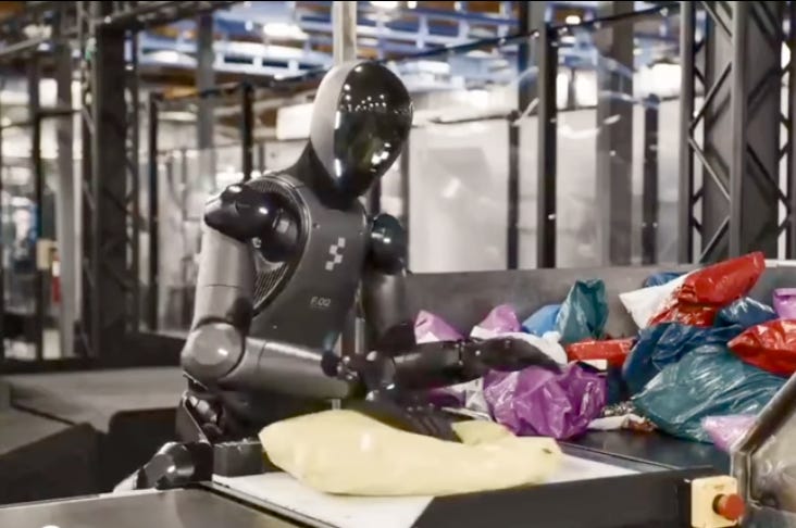
We’ve also seen some impressive-looking robotics demos over the last year, though these must be evaluated with a large grain of salt. Figure showed off its robots sorting packages for hours at a time and autonomously unloading a dishwasher. Physical Intelligence showed off its robot model making coffee and folding boxes in a chocolate factory. Generalist AI showed off its GEN-1.5 model learning new tasks from just a few examples.
Some progress in robots is a function of hardware advances: better actuators, and so on. But the lion’s share of it is due to advances in robot AI, using specially developed AI models to control a robot. As more general AI continues to rapidly advance in capabilities, one obvious question is whether we’re going to see the same sort of acceleration in robotic AI. Right now robotic AI capabilities still seem very limited, but given how fast more general AI improved, I can imagine this changing very quickly. Because of this, it’s worth understanding how the AI models being developed to control robots work.
There are a few different sorts of robotic AIs, which are sometimes referred to as “policies” (where a “policy” is something that maps a particular set of inputs — robot state, sensor data, instructions it’s been given — to a set of robot actions). For this essay, we’ll look at one commonly used architecture, employed by companies such as Figure, Unitree, Physical Intelligence, and Nvidia: the vision-language-action model (VLA). More specifically, we’ll look at one popular VLA, Physical Intelligence’s open-weight π0.5 VLA, which was released in 2025 and has become widely used (though it’s not Physical Intelligence’s most advanced model).
While a large language model takes text as an input and gives text as an output, a VLA takes text, images, and robot information as an input and gives a series of robot actions as an output. It does this using many of the same components that made LLMs so successful, specifically attention and the transformer architecture. It’s not amazingly obvious if VLA’s will remain the primary robotic AI paradigm, but as of now they’re a very common method for controlling robots.
Linear algebra basics
To learn how AI works (be it a VLA or anything else), it’s useful to know a very small amount of linear algebra. Specifically, we want to understand a few different operations for manipulating arrays of numbers, since this is most of what AI models do.
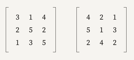
For instance, say we have the following two-dimensional arrays (or matrices) of numbers:
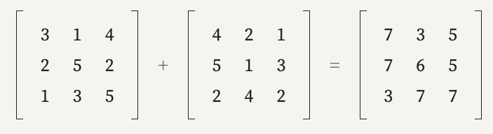
One thing we can do to these arrays is add them together. This works exactly like how you’d expect: each number in one array is added to the corresponding number in the other array, giving you a new array with all the resulting additions.
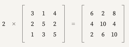
Another thing we can do is multiply or divide an array by a single value. This also works more or less like you’d expect: each value in the array gets multiplied or divided by the respective value.
But what if we want to multiply two matrices together? To do this, we need an operation called the dot product. The dot product takes two one-dimensional arrays of numbers (also known as vectors), multiplies each value in one vector by the corresponding value in the other vector, then sums the result.
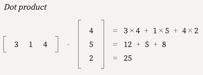
You can think of the dot product as measuring two things: how large two vectors are, and how similar they are to each other. (If you normalize the vectors, scaling the values so everything is between 0 and 1, then the dot product is entirely a measure of how similar two vectors are to each other.)
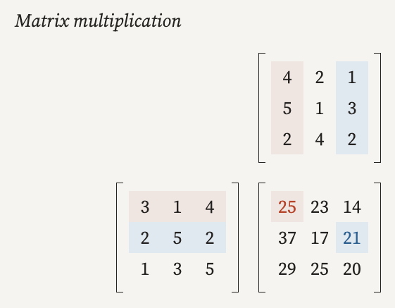
When we multiply two matrices together, we’re simply doing a bunch of dot products: each value in the resulting matrix is the dot product of the row of one array and the column of another. Because the dot product requires two lists of equal length, multiplication of matrices must be done in a certain way: the number of columns of one matrix must be equal to the number of rows of the other matrix. And the size of the output matrix will be a function of the sizes of the input matrices.
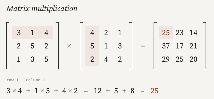
I find it easiest to understand matrix multiplication by putting one matrix on the left and the other matrix on the upper right. The output matrix fits in the space between them, each value the dot product of the first matrix’s rows and the second’s columns:
Neural network basics
Most modern AI models, as we know, are built using neural networks. The classic image of a neural network is something like this:
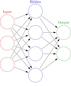
You have some series of input neurons that represent your input data, which are connected to various intermediate layers of neurons, which then get connected to output neurons. Depending on what data is fed into them and how the connections between different neurons have been set, neurons will “activate” to various degrees, taking some input from the neurons in the previous layer and sending some output along to the neurons in the next layer. This structure is sometimes called a “multilayer perceptron,” or MLP.
However, I think it’s much easier to understand neural networks by looking at how they’re actually implemented, which is done by multiplying arrays of numbers (in machine learning, these arrays are sometimes called “tensors,” where a tensor is just an array of numbers that can be any dimension. Google, for instance, has a machine-learning library called “TensorFlow”). The neural network above, for instance, would actually be implemented via something like this:
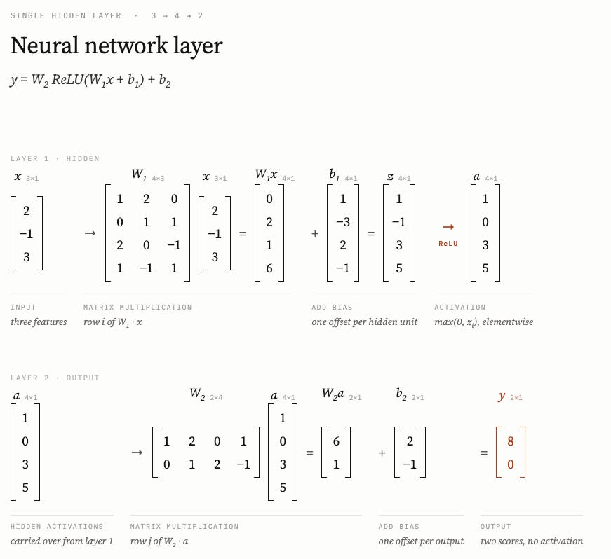
The three input neurons become a one-dimensional array, or vector, with three numbers in it, which is our input data. This vector then gets passed to the hidden layer, where it goes through several steps. First, it gets multiplied by a two-dimensional matrix (W1 in the figure). This matrix has four rows (corresponding to the four neurons in the original diagram) and three columns (one for each value in the input vector): it takes a vector three numbers long (or 3-vector) as an input and spits out one four numbers long as an output. The resulting vector of four numbers is then added to another 4-vector (b1 in the figure), the values of which are known as “biases.” The weights and biases of the various layers are known as the “parameters” of the network and are what get modified when the neural network is being trained.
Once the biases have been added, the resulting vector (known as a “pre-activation,” z in the figure) then goes through what’s called a nonlinearity, which is just a function that does different transformations to an input depending on what that input is. A common nonlinearity, which the example above uses, is “ReLU,” for rectified linear unit. All ReLU does is replace any negative numbers in the vector it’s given with zeroes. Other nonlinearities are the sigmoid (an S-shaped function that squeezes values to be between 0 and 1) and GELU (a somewhat ReLU-like function that’s smooth instead of sharply kinked).
In a basic MLP like this one, each hidden layer in a neural network will consist of this matrix multiplication, then bias, then nonlinearity. The network above has just one hidden layer, so after the nonlinearity the resulting vector is then passed to the output neurons. These transform the data again using another matrix multiplication (W2) and bias addition (b2), yielding a vector of two numbers as the output (y).
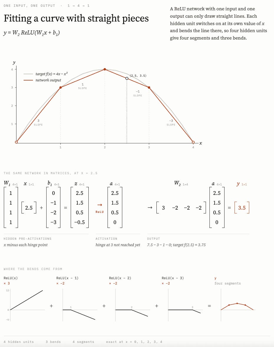
This structure is simple but powerful. To see why, imagine a neural network that takes a single value as an input and gives a single value as an output but has many neurons in its hidden layer (the number of neurons is known as the “width” of the layer). Before the nonlinearity, each individual neuron calculates wx + b, which is the formula for a straight line; the weights determine the slope of the line, while the biases determine its vertical location. The nonlinearity, in turn, lets the layer draw different line segments, with different slopes and intercepts, at different points on the graph. Together, this allows a sufficiently wide neural network to, in principle, approximate any continuous function by drawing a large number of different line segments1: the more hidden-layer neurons we add, the more line segments we can draw, and the closer we can approximate the function. In higher dimensions — larger numbers of inputs and outputs — the geometry gets more complicated, but the basic idea remains the same.
Training a neural network
Other than their ability to approximate very complex functions, the other key property of neural networks is that they can be trained, by comparing the actual output of a network to the output you’d like it to have, and nudging the weights and biases in response to make the output more accurate.
Training a network starts with a forward pass, giving it an example input and then calculating an output. This calculated output is then compared to the actual, correct output using some loss function, which measures the difference between the two. For a simple case where the output is a single number, the loss function might be mean squared error, which you can calculate by squaring the difference between the actual output and the expected output: the bigger the difference, the larger the loss. If you’re trying to predict the next symbol of a sequence, however, a common loss function is cross entropy, which is based on how likely the model thought the actual next symbol was; the less likely the model thought the correct symbol was, the higher the cross entropy. As a model gets trained and does a better and better job at approximating the correct output, the loss will (hopefully) trend downward, and reports on AI training runs will often show training loss curves.
Once the loss has been determined, the next step is to go back through the network, layer by layer, and, using the chain rule, calculate how much the loss would change if you made small adjustments to each weight and bias. This is known as backpropagation and produces a long list of numbers, each number telling you how much the loss would change when you adjust the value of one parameter in the model. This list, called the gradient, can be thought of as the direction you’d need to “step” in a high-dimensional space to maximally increase the loss for the current values of the model’s parameters.
The gradient in hand, the next step is to take a small step in the opposite direction (since we want to decrease the loss, not increase it). This is done by multiplying each value in the gradient by a small positive number (known as the learning rate), and then subtracting the resulting number from each parameter. With the parameters changed, you can then run another input through the model, calculate the new loss, and modify the parameters again. This process of repeatedly calculating the gradient, then using it to modify the parameters of the model to (hopefully) reduce the loss is known as gradient descent.
In practice, most models are trained using modified, more complex versions of gradient descent that do things like use the average of recent gradients to update the parameters and use different learning rates at different points in the training process. It’s also uncommon in practice to update the model after every individual training example. Models are instead trained in batches (sometimes called “minibatches”): dozens, hundreds, or even more training examples are run through the model, their losses are averaged, and the gradient is calculated based on the average loss. Settings that determine how a model is trained, such as learning rate or batch size, are known as “hyperparameters,” and figuring out the best hyperparameters to train a model with is an important area of machine learning.
Inputs to a neural network
For an AI to do useful work, we’d like to be able to feed it things like images and text data. How do we convert images, text, and other data into a form that a model can understand and operate on?
For text, there are two main steps. First, a string of text is broken up into chunks, or “tokens.” Then, each token is converted into a long vector of numbers, called an “embedding,” which can then be processed by the network. Let’s take each step in turn.
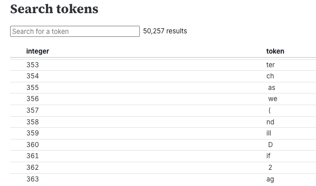
Tokenizing is a way to break a string of text into a series of chunks, which is useful because it allows the model to learn something about the meaning of individual chunks of text. One option would be to break apart text using a predefined list of words, but a fixed list of whole words would prevent us from processing words or character combinations that haven’t been seen before. So instead it’s more common to use token libraries, which contain both individual characters and clusters of characters (including whole words as well as portions of words) that have been found to occur frequently in actual bodies of text. The token vocabulary for GPT-3, for instance, has around 50,000 items in it. You can browse the GPT token vocabulary here and see that it contains individual characters, chunks of words, and entire words (often with punctuation or spaces included).
Once a text is broken up into individual tokens, each token then gets converted into an embedding, a long vector of numbers. The embedding vector for GPT-3, for instance, is 12,288 numbers long. You can think of this embedding vector as representing coordinates in some very high-dimensional space. The conversion is done using an embedding matrix, which is effectively a huge matrix where each row is the embedding for one particular token. The image below shows an example of converting the string “the cat sat on the mat” to a series of embedding vectors using a (highly simplified) token vocabulary and embedding table.
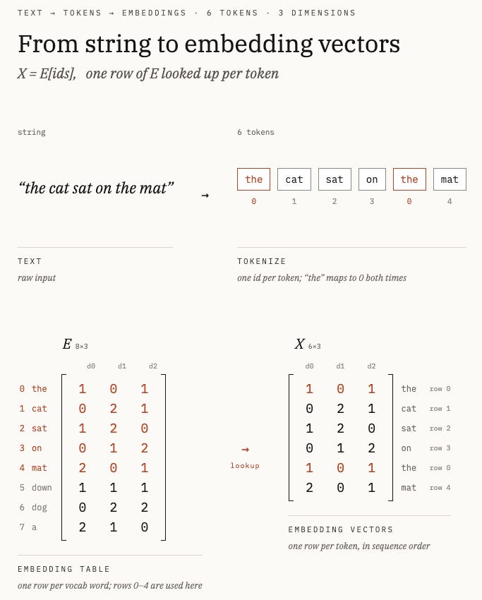
One key fact about the embedding matrix is that the values in it — the numbers in each embedding vector — are model parameters that are learned, just like the weights and biases in a multilayer perceptron. As a model is trained, the embedding vectors will get updated via whatever flavor of gradient descent is being used, and tokens that the model learns are similar or even substitutable might end up closer to each other in “embedding space.”
With images, we can use a similar process, but it must be modified somewhat. In something like a vision transformer (an AI model used for things like image classification), an image is first broken into a series of smaller chunks (say, a square of 16 × 16 pixels) called patches, the image equivalents of tokens. However, unlike with tokens, it’s not feasible to have a unique embedding vector for every possible image patch, because the number of possible patches is too large. Even if an image was limited to just black and white pixels, the number of unique 16 × 16 patches is 2^256, which is not all that much less than the estimated number of atoms in the universe. This is far too many items to list in a table.
Instead, patches are converted to embedding vectors using a learned embedding function. A patch is first converted to a very long vector containing the numerical color values of each pixel. This vector is then converted to an embedding vector using some learned embedding function (such as multiplying by a learned matrix), the parameters of which are updated via training.
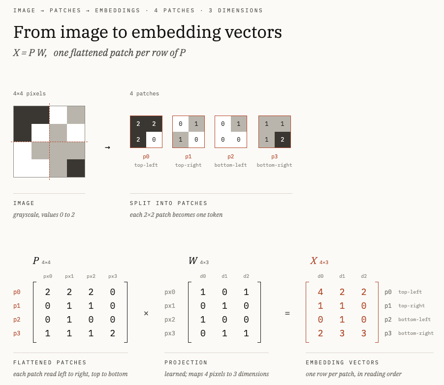
For both text and images, this process produces a matrix, where each row is an embedding vector for one particular token or patch. Because the embedding vector on its own doesn’t give any information on where a token occurs in a particular bit of text, the list of embedding vectors is often modified by adding a position-encoding vector to each embedding vector.
Attention and the transformer
Sticking with text for a moment, we have our tokenizer and embedding matrix, which convert words into long vectors of numbers. We add position information to those vectors, and then feed them into a neural network, modifying them in various ways and eventually producing some output.
One weakness of this arrangement is that while the network can learn about the general similarities of various chunks of text by way of the embedding table, embedding vectors don’t include any information about what a token means in a particular string of text. The vectors for the tokens “red” and “crimson” will reflect what the model has learned about how these are used generally, and since they describe similar colors they might end up with similar embedding vectors near each other in embedding space. But this won’t give any information about what they mean in a sentence like “the harvard crimson staff were seeing red on sunday when the president shut down their office.” If we want to accurately predict the next token in a sequence of them, it would be useful if we could modify the embedding vectors to include information about the surrounding context.
One way of doing this that has proved to be very successful is called “attention.” Attention is basically a way to modify an embedding vector with information about its surrounding context. This is done by turning the embedding vector for a token into three other vectors: a query vector, a key vector, and a value vector. Each one is created by multiplying the embedding vector by some matrix. As with the embedding table, these matrices are learned: the values in them will be modified via the training process. In GPT-3, the query, key, and value vectors are each 128 numbers long.
The query vector can be thought of as representing something like “what other tokens are important for interpreting me?” The key vector can be thought of as representing something like “what sort of thing am I useful for?” And the value vector can be thought of as representing “what sort of information will I provide?” The resulting vectors are combined together in a query matrix Q, a key matrix K, and a value matrix V, each row the vector for some particular token.
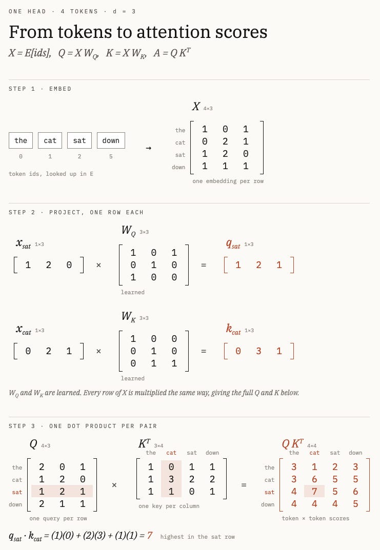
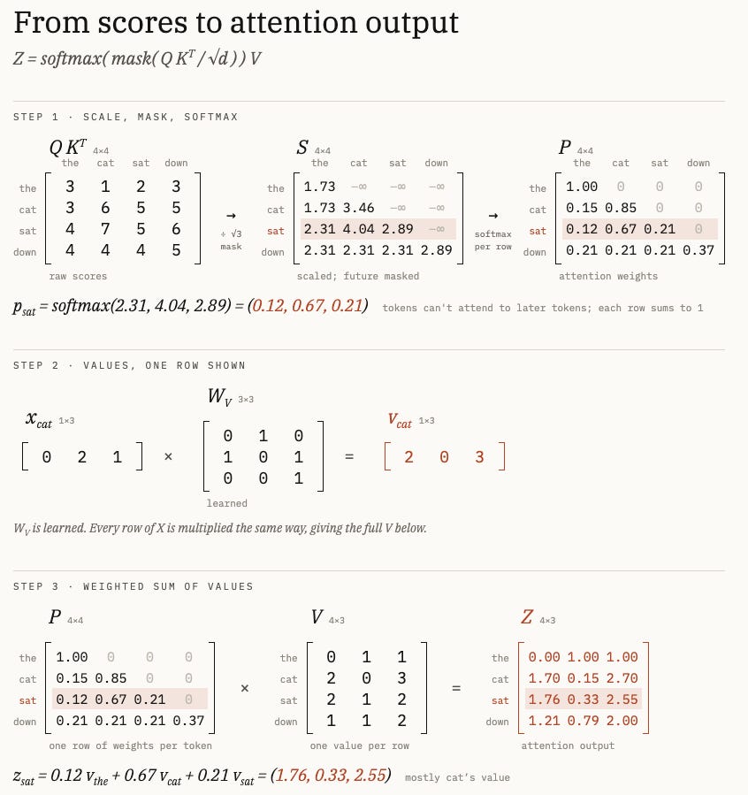
To calculate attention, the query matrix Q is multiplied by the transposed key matrix K (where “transposed” means “rows turned into columns and vice versa”). This gives a new matrix, QKᵀ, whose values indicate how important each token is for understanding every other token. There are then a few mechanical steps done to this matrix. First, we divide each value in the QKᵀ matrix by the square root of the length of the key vector, to prevent the values from getting too large. When predicting the next token in a sequence, we don’t want earlier tokens to be able to “see” later ones. We correct this by what’s called “causal masking” — essentially setting the values for later tokens on earlier ones to negative infinity. We also scale the values in each row so that they’re between 0 and 1 and sum to 1, using a function called “softmax.” (If you had the vector [10 6 4], softmax would convert it to [0.5 0.3 0.2]). You can think of this as creating a matrix that tells us how much information each token should take from other tokens.
The scaled, masked QKᵀ matrix is then multiplied by the value matrix V. The output of this multiplication is a list of embedding vectors, where each vector has been modified to have information about the token’s surrounding context.
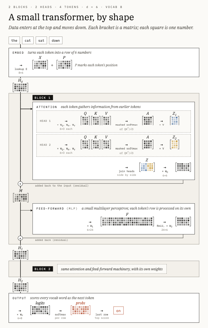
In practice, it’s common to run this attention mechanism multiple times simultaneously (this is called “multiple attention heads”). GPT-3, for instance, has 96 attention heads. Each attention head learns different matrices for calculating Q, K, and V, and might learn different things to look for in the surrounding context: you can imagine one attention head “looking” for related nouns, one looking for previous mentions of a word, and so on. (These are just conceptual examples; in practice the things an attention head learns to “attend to” don’t necessarily map cleanly to concepts like this.) The output of each attention head will get stitched together into one matrix, which then gets multiplied by another learned matrix, which mixes the information from different heads together. The resulting matrix can then get processed by the rest of the neural network.
Probably the most common way to use attention is via what’s called the transformer architecture. A GPT-style transformer consists of multiple “transformer blocks,” each one of which contains an attention step followed by a multilayer perceptron. GPT-3, for instance, contains 96 transformer blocks. In the first transformer block, the model is fed the embedding vectors for the tokens, which are then processed by the 96 attention heads, producing an output matrix whose rows are modified and processed embedding vectors. Each row of the matrix then goes through an MLP with a single hidden layer of neurons: while the attention mechanism mixes information between tokens, the MLP processes each embedding vector it receives separately, modifying them further. The output then gets fed into another transformer block, which does the same thing: running the attention mechanism over the output from the previous block (using totally new learned matrices for calculating Q, K, and V), then sending it to an MLP. This is done again and again, through all the transformer blocks, until at the end the vector for the last token is converted into a list of scores, one for each possible token, representing the model’s guess at how likely each token is next in the sequence.
Vision, language, action
A transformer architecture can also be used to process images. The Vision Transformer (ViT) base model described in a 2020 paper by a team from Google uses 12 transformer blocks, each one with 12 attention heads. One difference with the vision transformer is that there’s no causal masking: every token can “see” every other token when processed by the attention mechanism. Another difference is the output: while a GPT-style language transformer takes a string of tokens as an input and predicts the next token as an output, the initial vision transformer takes a string of image “tokens” as an input and produces a classification of the image as an output.
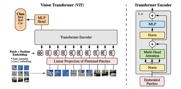
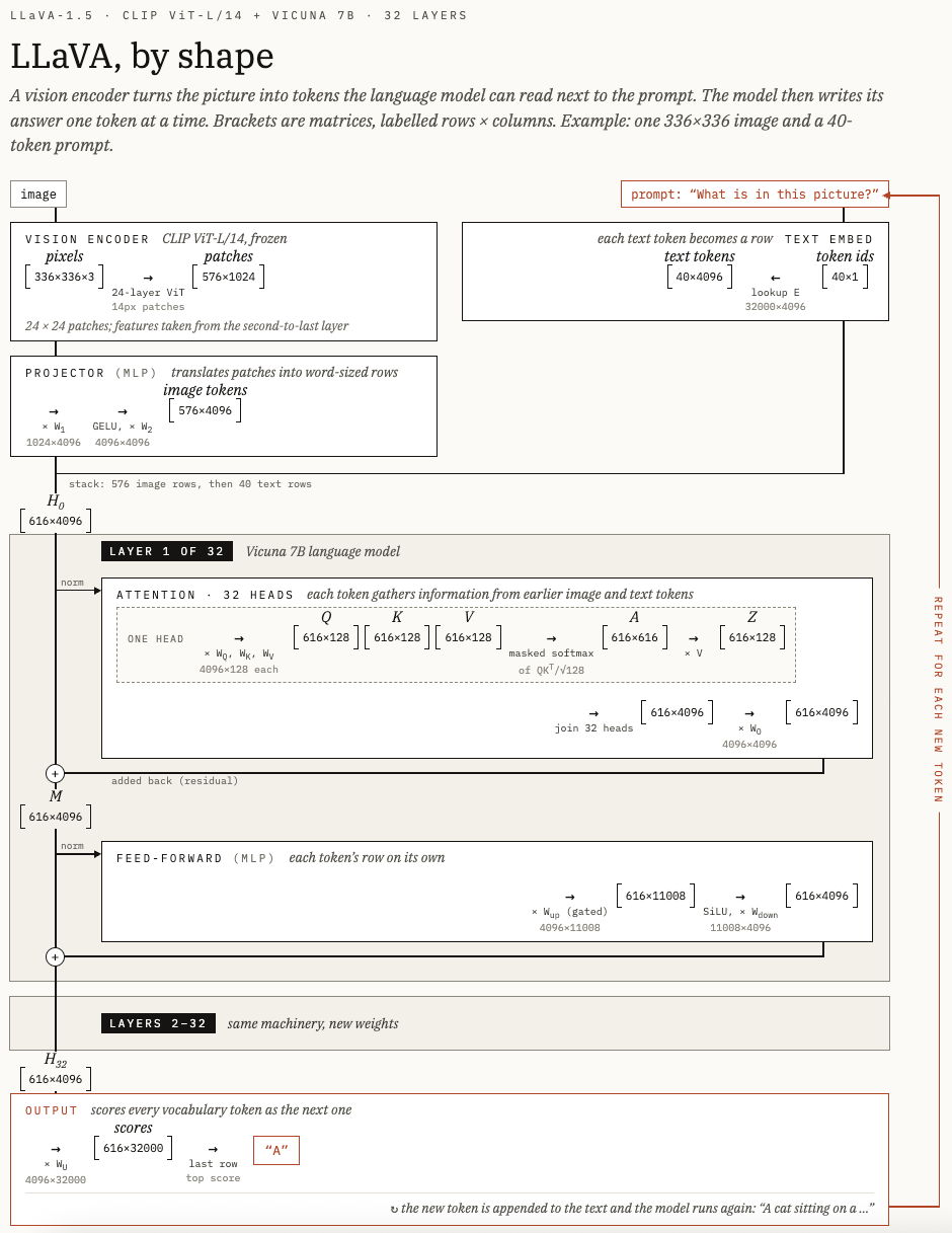
With a transformer capable of processing vision or text, it’s not much of a leap to design one that can process BOTH image and text: say by feeding it an image and a text query (“What is this a picture of?”) and having the model generate an answer. This is known as a vision-language model, or VLM. LLaVA (short for Large Language and Vision Assistant) is one such model. In LLaVA-1.5, an image is fed into a vision transformer, which breaks it into patches, converts those patches into embeddings, and then sends the embeddings through a series of vision transformer blocks, producing a series of vectors (one for each patch). Those vectors then get converted via what’s known as a “projector,” an MLP that changes their size and modifies their representation into something that an LLM expects. These converted vectors then get fed, along with embeddings from the input text tokens, into an LLM, which consists of another series of transformer blocks. Attention in this transformer can look at both the vectors from the image and text, modifying them based on what’s in the image and what’s in the text. The data flows through the transformer blocks, eventually getting spit out as a predicted string of text (“It’s a picture of a dog”). This basic architecture — a vision transformer, a projector that converts its output into LLM-sized vectors, and then an LLM that processes the text and image data — is common, though various models implement it in different ways.
You can similarly use a transformer architecture to drive a robot, by feeding it information on robot state along with images and text, and having it output a series of robot actions. This is called a vision-language-action model, or VLA. The architecture for the π0.5 VLA is shown in the image below:
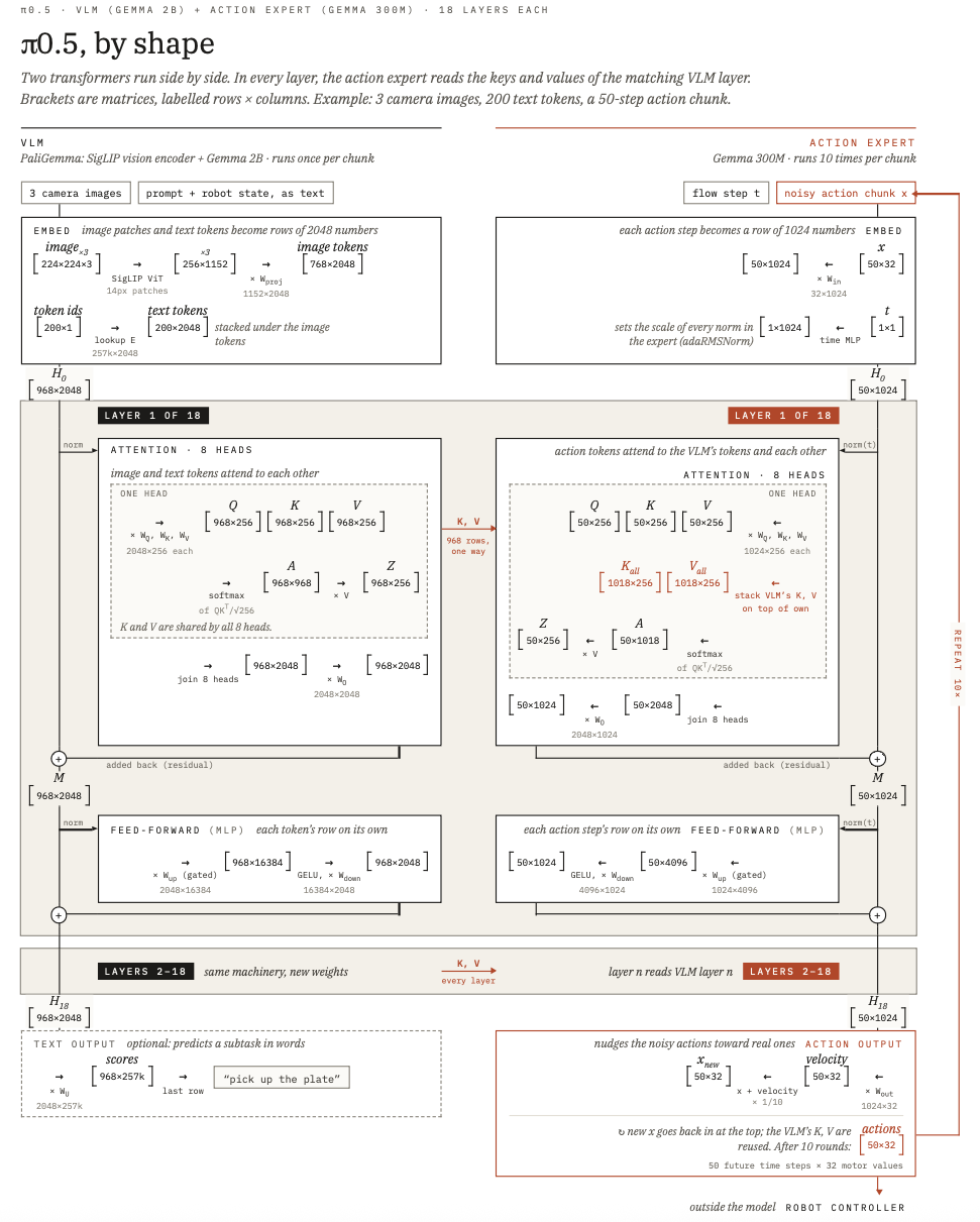
Image data from the robot’s cameras, text instructions, and data representing the robot’s state are all converted into token embeddings via various encoders. These then get fed into a language backbone, which consists of a series of 18 transformer blocks. (Interestingly, these have multiple attention heads, but ONLY for the query matrix: the key and value matrices are the same for each attention head. This is called “multi-query attention.”)
Running in parallel with this vision-language model is another transformer, the action transformer, which also consists of 18 transformer blocks (the same as the vision-language model). This action transformer gets fed an input of token embeddings representing essentially 50 random actions. These make their way through the transformer, and at each attention step for each action vector the action transformer looks not only at the other action vectors, but at the vectors from the images, text, and robot state at the corresponding block in the vision-language model. It then modifies those action embeddings, moving them away from random actions based on the information that it obtains from the text and image vectors. As the action vectors make their way through the action transformer, they continue to be modified using information from the processed image, text, and state vectors. The output of the action transformer then gets used to correct the input “noise” actions, and the whole process runs again. After 10 iterations, the output of the action transformer is, hopefully, a useful sequence of 50 actions. (The model processes 50 actions at a time because outputting a single action, and then running the entire model again for the next action, would make the robot move very slowly. This is called “action chunking.”) These actions take the form of joint-angle or gripper-position targets, which then get fed into a traditional robot controller that converts them into motor torques to actually move the robot.
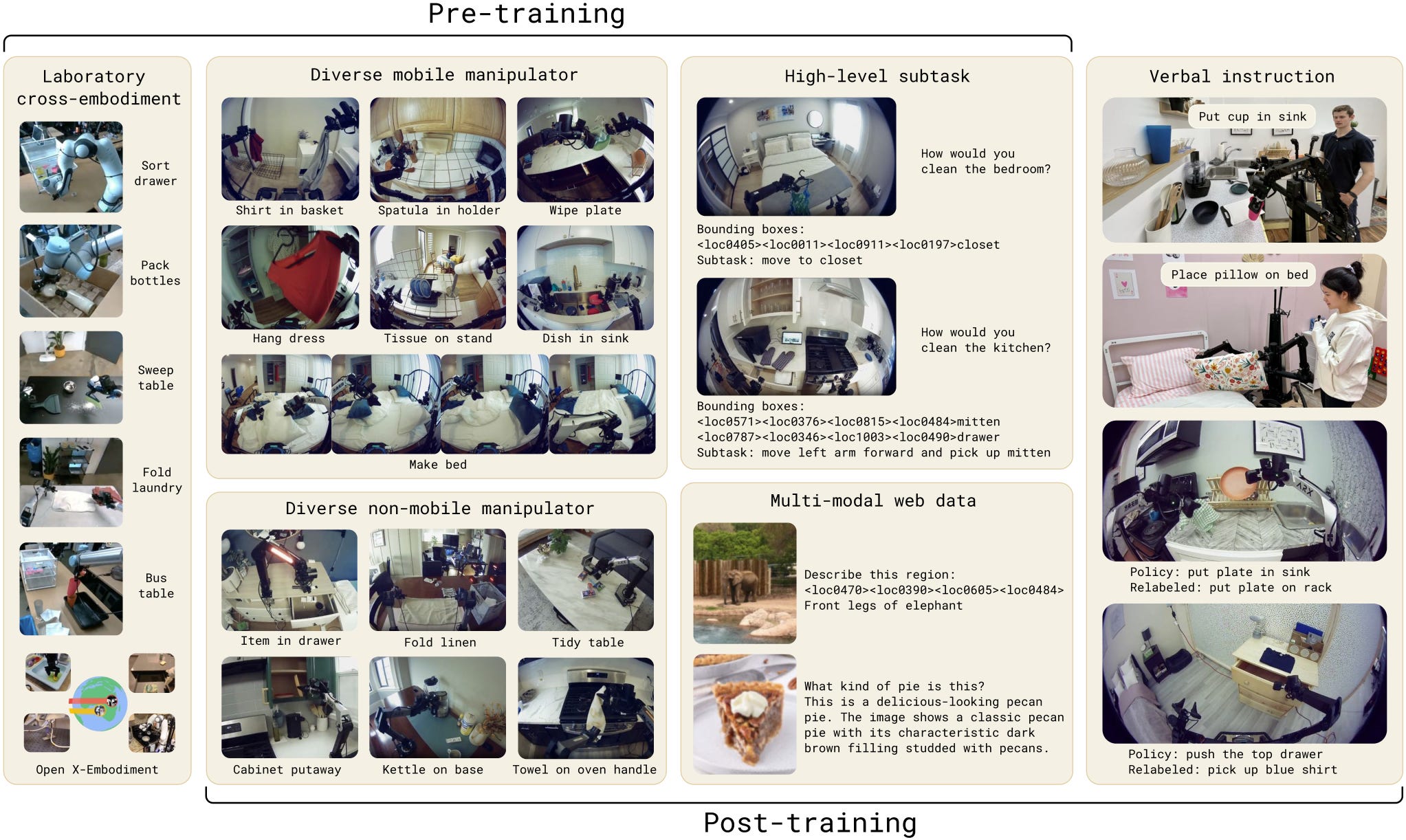
This system was assembled from various pre-existing components and then trained together. The transformer that converts image patches into embedding vectors is called SigLIP, a 400-million-parameter model first created in 2023 and trained on pairs of images and text. In 2024, Google combined SigLIP with an existing, 2-billion-parameter LLM called Gemma (which had been trained on 3 trillion tokens of text) to create the PaliGemma VLM, which was then further trained on over a billion training examples. These examples included tasks like captioning images and answering questions about them. To create the π0.5 VLA, Physical Intelligence took PaliGemma, combined it with a system for converting robot actions into tokens (which they call FAST) and a newly created action transformer (a 300-million-parameter model), and then trained the combined system on various robotic manipulation tasks (as well as some additional image description tasks).
Conclusion
Before looking into this I knew, vaguely, that robot AI models were similar to the models used for AI chatbots that I was familiar with. But I was struck by how much overlap between the two is, with VLAs literally using LLMs trained on text as a major building block, and the basic transformer architecture from LLMs being applied to generate robot actions. This doesn’t necessarily mean that we’ll see the same sorts of rapid improvements with robot capabilities that we’ve seen with AI more generally, but it does make me think it might be possible.
Robots and the AI that controls them is something that I expect to become increasingly important, and it’s a subject I plan on spending more and more time on, with more and deeper looks at the technology and how it’s progressing.
Over a fixed, bounded range of inputs.
Thanks! That is the most complete description of how these systems work I've seen. May I ask what additional functionality is hoped for by the use of all these enormous data centers that are being constructed. Is it mostly aimed at robotics or what? LLM's by themselves already seem maxed out or very nearly so.
Worth stating what the reuse means commercially. A robotics company's capability curve is now set by a 2B parameter backbone somebody else trained on 3T tokens. That is not a technology choice. It is a supplier relationship. The saving is real and so is the dependency. Firms in this position tend to find out what the vendor can charge only after switching has become expensive.